Cluster
Purpose
Hierarchical Cluster Analysis with dendrograms.
Synopsis
- [results,fig] = cluster(data,labels,options)
- [results,fig] = cluster(data,options)
Description
cluster(data) performs unsupervised hierarchical cluster analysis (HCA) on the input data data, using one of several different clustering methods, defined in the options structure.
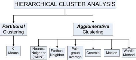
Cluster Analysis methods can be classified into two main categories: agglomerative and partitional. Agglomerative methods begin with each object being it's own cluster, and proceed to combine (agglomerate) the closest clusters into larger ones. Partitional methods start with a single cluster containing all objects, and proceed to divide the objects into additional clusters.
The cluster function enables six different agglomerative methods (Nearest Neighbor, Furthest Neighbor, Pair Group Average, Centroid, Median and Ward's Method) and one partitional method (K-means).
All clustering methods require the specification of a distance measure to be used to indicate distances between objects, and subsequently between clusters, during method operation. First, one could use either the original X-variables or PCA scores to determine the distance. The usage of PCA scores can provide colinearity and noise-reduction benefits, but requires the specification of the appropriate number of PCsd. Additionally, given the input variables (X-variables or PC scores) one can then choose either the Euclidean or the Mahalanobis distance to complete the definition of the distance measure. The use of Mahalanobis distance allows one to account for dominant multivariate directions in the data when performing cluster analysis.
The K-means partitional clustering method starts with a random selection of K objects that are to be used as cluster targets, where K is determined a priori. During each cycle of this clustering method, the remaining objects are assigned to one of these clusters, based on distance from each of the K targets. New cluster targets are then calculated as the means of the objects in each cluster, and the procedure is repeated until no objects are re-assigned after the updated mean calculations.
All of the agglomerative methods start with each object defining it's own cluster. Then, each cycle of the method involves calculation of all inter-cluster distances based on the specified
File:Cluster Methods Table.jpg
Optional input labels can be used to put labels on the dendrogram plots. For data M by N then labels must be a character array with M rows. When labels is not specified and data is class "double", the dendrogram is plotted using sample numbers. When labels is not specified and data is a DataSet object, the dendrogram is plotted using sample labels included in the DataSet object. If the DataSet labels field is empty it will use sample numbers.
The output is a dendrogram showing the sample distances.
Note: Calling cluster with no inputs starts the graphical user interface (GUI) for this analysis method.
Outputs
- results = a structure containing results of the clustering (defined below)
- fig = the handle to any plot created.
The results output containing the following fields:
- dist : the distance threshold at which each cluster forms.
- class : the classes of each sample (columns of class) for each distance (rows of class).
- order : the order of the samples which locates similar samples nearest to each other (this is the order used for the plots).
- linkage : a table of linkages where each row indicates a linkage of one group to another. Each row in the matrix represents one group. The first two columns indicate the sample or group numbers which were linked to form the group. The final column indicates the distance between linked items. Group numbers start at m+1 (where m is the number of samples in the input dat matrix) thus, row j of this matrix is group number m+j. This matrix can be used with the statistics toolbox dendogram function.
The (results.class) matrix can be used with the (results.dist) matrix to determine clusters of samples for any distance using:
  results   = cluster(data);                      %do cluster
  ind       = max(find(results.dist<threshold));  %user-desired threshold
  thisclass = results.class(ind,:);               %grab arbitrary classes
Options
options = a structure array with the following fields:
- plots : ['none' | {'final'} ] Governs plotting. When set to 'none', the distance/cluster matrix is returned, 'final' returns a dendrogram plot showing sample distances.
- algorithm: [ ] clustering algorithm. May be one of the following:
- knn : K-Nearest Neighbor {DEFAULT}
- fn : Furthest Neighbor
- avgpair : Average Paired Distance
- med : Median
- cnt : Centroid
- ward : Ward's Method
- kmeans : K-means
- preprocessing : {[ ]} Preprocessing structure or keyword (see PREPROCESS),
- pca : [ {'off'} | 'on' ] if 'on' then CLUSTER performs PCA first and clustering on the scores,
- ncomp : [ ] number of PCA factors to use {default = [ ], the user is prompted to select the number of factors from the SSQ table},
- mahalanobis : [ {'off'} | 'on' ] if 'on' then a Mahalanobis distance on the scores is used,
- slack : [0] integer number indicating how many samples can be "overridden" when two class branches merge. If the smaller of the two classes has no more than this number of samples, the branch will be absorbed into the larger class. This feature is only valid when classes are supplied in the input data. A value of 0 (zero) disables this feature.
