DataSet Construction
Getting Started
In general, the Dataset Object (DSO) is a MATLAB object for containing an array of numeric data along with auxiliary information, or metadata, pertaining to the data itself. This metadata could consist of (including but not limited to): sample names, variable labels, class labels, time and/or wavelength axes. See these pages for an overview on the DSO:
From a GUI
Using PLS_Toolbox and Solo, it is more convenient to import a file as a dataset object using the data importer. From the workspace browser, select File -> Import Data to launch the Import GUI.
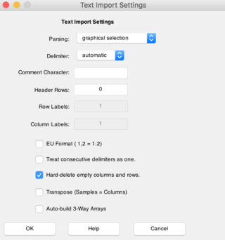
Alternatively, the Import GUI can be initialized by dragging the desired file into the Workspace Browser. In the case of text based file formats such as CSV or TXT, this will launch the Text Import Settings window.
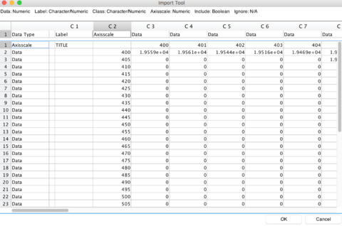
The Text Import Settings window allows to set various options specific to file that is being imported. Some of these settings include the number of header rows to ignore and the designated delimiter character. Clicking OK will launch the data Import Tool GUI shown below. The user can then designate which columns and rows to be used as axisscales, labels, etc. In this example, the first column has been specified as ‘Label’ and the first row and the second column have both been specified as axisscales.
From the MATLAB Command Line
DSOs can be created by passing an array to the DSO constructor method 'dataset()'. In this example, we loaded one of several demo DSOs, provided with PLS_Toolbox/Solo called 'wine' to extract the data for the purpose of demonstrating how to create a new DSO. 'wine' contains 10 samples (labeled as countries) and 5 measurements regarding alcohol consumption (wine, beer, and liquor), as well as life expectancy and heart disease.
Extracting the data from the DSO is done by referencing its '.data' field and assign a copy of the data into a new variable 'dat'. Conversely we can extract other fields in the DSO by referencing them in a similar manner; The sample names (named 'country' in 'wine'), and measurement labels are stored in .label{1} and .label{2}, respectively. Note that the '.label' field is a cell array and the labels for the samples are always stored in the first element while labels for measurements are always stored in the second element. When more than one label set is present the respective providing a second index value ('.label{1,2}').
» load wine
» dat   = wine.data;
» names = wine.label{1};
» vars  = wine.label{2};
» whos
  Name        Size            Bytes  Class      Attributes

  dat        10x5               400  double
  names      10x6               120  char
  vars        5x6                60  char
  wine       10x5             12156  dataset
Once the data, measurement labels, and sample labels have been obtained (and stored in the variables 'dat', 'names', & 'vars', respectively), a new dataset can be constructed. We may also provide a new name, authorship, and description which are stored in their respective fields ('.name', '.author', and '.description').
» wined = dataset(dat);
» wined.name = 'Wine';
» wined.author = 'A.E. Newman';
» wined.description= ...
{'Wine, beer, and liquor consumption (gal/yr)',...
'life expectancy (years), and heart disease rate', ...
'(cases/100,/yr) for 10 countries.'};
» wined.label{1} = names;
» wined.label{2} = vars;
Additional assignments, such as labels, titles, axisscale for the first mode (rows/samples), can be made by explicitly indexing them as shown below:
» wined.labelname{1} = 'Countries';
» wined.label{1} = ...
{'France' ...
'Italy', ...
'Switz', ...
'Austra', ...
...
'Mexico'};
» wined.title{1} = 'Country';
» wined.class{1} = [1 1 1 2 3];
» wined.classname{1} = 'Continent';
» wined.axisscale{1} = 1:5;
» wined.axisscalename{1} = 'Country Number';
Conversely, additional assignments can be made for the second mode (columns/measurements) by explicitly indexing them as shown below:
» wined.labelname{2} = 'Variables';
» wined.label{2} = ...
{'Liquor','Wine','Beer','LifeExp','HeartD'};
For N-way DSOs, the assignment process is extended to the other modes by referencing the targeted mode. Moreover, the labels and axissscales can be further extended by creating new sets of labels/axisscales by providing a second index value:
» wined.labelname{2,2} = 'Alcohol Content and Quality';
» wined.label{2,2} = {'high','medium','low','good','bad'};
Individual labels can be replaced by indexing to a given label set by using a second curly bracket {} followed by the assignment operator:
» wined.label{2,2}{4} = 'excellent';
Creating 3-Way Data
Like the 2-way DSO, there are several ways to create a 3-way DSO in PLS_toolbox: from the GUI and from the MATLAB Command Line.
From a GUI
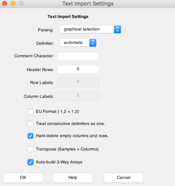
If the data is given in separate text-based files such as .csv, the data can easily be imported into a 3-way DSO using the Text Import tool. This is done by dragging multiple files into the Workspace Browser and then checking the ‘Auto-build 3-way Arrays’ checkbox option in the Text Import Settings window.
From the MATLAB Command Line
Constructing a 3-way DSO via Command Line can be a bit more involved depending on the data. If the data is already stored in a 3-way array of type double, simply declare a new DSO using said array:
» dso3way = dataset(x3way);
For constructing a 3-way DSO from several 2-way arrays (or DSOs), there are several issues to consider: labels, axisscales, etc., but most importantly is modes 1 and 2 of data (arrays or DSOs) must have of same lengths (i.e., the same number of elements).
Consider several 2-way arrays (a 2x10, and corresponds to a single sample). A new DSO should be declared and initialized and with the first mode corresponding to sample and the second and third correspond to the measurements. Further samples may be appended as shown:
» dso3way = dataset(zeros(3,2,10));
» dso3way.data(1,:,:) = x1;
» dso3way.data(2,:,:) = x2;
» dso3way.data(3,:,:) = x3;
» dso3way.data(4,:,:) = x4; % Appended


