Advanced Preprocessing: Noise, Offset, and Baseline Filtering: Difference between revisions
imported>Jeremy |
No edit summary |
||
| Line 30: | Line 30: | ||
'''Figure''': NIR spectra of corn (A), the first derivative of the spectra (B), and the second derivative of the spectra (C). | '''Figure''': NIR spectra of corn (A), the first derivative of the spectra (B), and the second derivative of the spectra (C). | ||
[[Image: | [[Image:App_savgol_1_lwl.png|500px|]] | ||
Note that at the end-points (and at excluded regions) of the variables, limited information is available to fit a polynomial. The SavGol algorithm approximates the polynomial in these regions, which may introduce some unusual features, particularly when the variable-to-variable slope is large near an edge. In these cases, it is preferable to exclude some variables (''e.g.'', the same number of variables as the window width) at the edges. | Note that at the end-points (and at excluded regions) of the variables, limited information is available to fit a polynomial. The SavGol algorithm approximates the polynomial in these regions, which may introduce some unusual features, particularly when the variable-to-variable slope is large near an edge. In these cases, it is preferable to exclude some variables (''e.g.'', the same number of variables as the window width) at the edges. | ||
Revision as of 16:35, 18 September 2019
Introduction
A variety of methods exist to remove high- or low-frequency interferences (where frequency is defined as change from variable to variable). These interferences, often described as noise (high frequency) or background (low frequency) are common in many measurements but can often be corrected by taking advantage of the relationship between variables in a data set. In many cases, variables which are "next to" each other in the data matrix (adjacent columns) are related to each other and contain similar information. These noise, offset, and baseline filtering methods utilize this relationship to remove these types of interferences.
Noise, offset, and baseline filtering methods are usually performed fairly early in the sequence of preprocessing methods. The signal being removed from each sample is assumed to be only interference and is generally not useful for numerical analyses. One exception to this is when normalization is also being performed. In these cases, it sometimes occurs that a background or offset being removed is fairly constant in response and is, therefore, useful in correcting for scaling errors. For more information, see the normalization methods described below.
Note that these methods are not relevant when working with variables which do not have this similarity, such as process variables, genetic markers, or other highly selective or discrete variables. For such variables, use of multivariate filtering methods (described later) may be of use for removing interferences.
Smoothing (SavGol)
Smoothing is a low-pass filter used for removing high-frequency noise from samples. Often used on spectra, this operation is done separately on each row of the data matrix and acts on adjacent variables. Smoothing assumes that variables which are near to each other in the data matrix (i.e., adjacent columns) are related to each other and contain similar information which can be averaged together to reduce noise without significant loss of the signal of interest.
The smoothing implemented in PLS_Toolbox is the Savitzky-Golay (SavGol) algorithm (Savitzky and Golay, 1964). The algorithm essentially fits individual polynomials to windows around each point in the spectrum. These polynomials are then used to smooth the data. The algorithm requires selection of both the size of the window (filter width) and the order of the polynomial. The larger the window and lower the polynomial order, the more smoothing that occurs. Typically, the window should be on the order of, or smaller than, the nominal width of non-noise features.. Note that the same algorithm is used for derivatives (see below) and can be converted from one into the other by changing the derivative order setting.
From the command line, this method is performed using the savgol function.
Derivative (SavGol)
Derivatives are a common method used to remove unimportant baseline signal from samples by taking the derivative of the measured responses with respect to the variable number (index) or other relevant axis scale (wavelength, wavenumbers, etc.) Derivatives are a form of high-pass filter and frequency-dependent scaling and are often used when lower-frequency (i.e., smooth and broad) features such as baselines are interferences and higher-frequency (i.e., sharp and narrow) features contain the signal of interest. This method should be used only when the variables are strongly related to each other and adjacent variables contain similar correlated signal.
The simplest form of derivative is a point-difference first derivative, in which each variable (point) in a sample is subtracted from its immediate neighboring variable (point). This subtraction removes the signal which is the same between the two variables and leaves only the part of the signal which is different. When performed on an entire sample, a first derivative effectively removes any offset from the sample and de-emphasizes lower-frequency signals. A second derivative would be calculated by repeating the process, which will further accentuate higher-frequency features.
Because derivatives de-emphasize lower frequencies and emphasize higher frequencies, they tend to accentuate noise (high frequency signal). For this reason, the Savitzky-Golay algorithm is often used to simultaneously smooth the data as it takes the derivative, greatly improving the utility of derivatized data. For details on the Savitzky-Golay algorithm, see the description for the smoothing method, above.
As with smoothing, the Savitzky-Golay derivativization algorithm requires selection of the size of the window (filter width), the order of the polynomial, and the order of the derivative. The larger the window and lower the polynomial order, the more smoothing that occurs. Typically, the window should be on the order of, or smaller than, the nominal width of non-noise features which should not be smoothed. Note that the same algorithm is used for simple smoothing (see above) and can be converted from one into the other by changing the derivative order setting.
An important aspect of derivatives is that they are linear operators, and as such, do not affect any linear relationships within the data. For instance, taking the derivative of absorbance spectra does not change the linear relationship between those data and chemical concentrations.
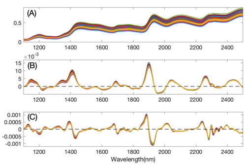
The figure below shows the results of first and second derivativization on the near-IR spectra of corn. Notice that taking the first derivative has removed the predominant background variation from the original data. The smaller variations remaining are due to the chemical differences between samples.
Figure: NIR spectra of corn (A), the first derivative of the spectra (B), and the second derivative of the spectra (C).
Note that at the end-points (and at excluded regions) of the variables, limited information is available to fit a polynomial. The SavGol algorithm approximates the polynomial in these regions, which may introduce some unusual features, particularly when the variable-to-variable slope is large near an edge. In these cases, it is preferable to exclude some variables (e.g., the same number of variables as the window width) at the edges.
From the command line, this method is performed using the savgol function.
Detrend
In cases where a constant, linear, or curved offset is present, the Detrend method can sometimes be used to remove these effects (see, for example, Barnes et al., 1989).
Detrend fits a polynomial of a given order to the entire sample and simply subtracts this polynomial. Note that this algorithm does not fit only baseline points in the sample, but fits the polynomial to all points, baseline and signal. As such, this method is very simple to use, but tends to work only when the largest source of signal in each sample is background interference.
In measurements where the variation of interest (net analyte signal) is a reasonably significant portion of the variance, Detrend tends to remove variations which are useful to modeling and may even create non-linear responses from otherwise linear ones. In addition, the fact that an individual polynomial is fit to each spectrum may increase the amount of interfering variance in a data set. Due to these reasons, use of Detrend is recommended only when the overall signal is dominated by backgrounds which are generally the same shape and are not greatly influenced by chemical or physical processes of interest. In general, derivatives tend to be far more amenable to use before multivariate analysis.
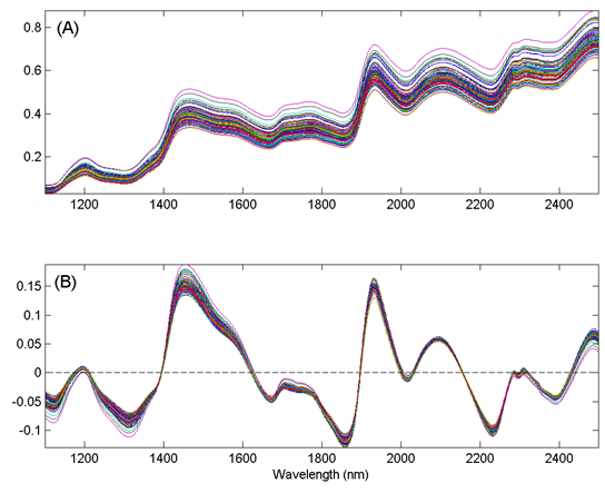
The figure below shows the effect of Detrend on the corn near-IR data. Note that the general linear offset is removed from all spectra, giving a mean intensity of zero for each spectrum.
Figure: The effect of first-order detrending on the corn near-IR spectral data. The original data are shown in (A) and the detrended data in (B).
The single setting for Detrend is the order of polynomial to fit to the data.
From the command line, there is no specific function to perform Detrend (although there is a MATLAB function of the same name). However, this method can be performed using the baseline function by indicating that all points in the spectrum are to be used in the baseline calculation.
Baseline (Specified points)
The specified points baseline method allows the user to fit a polynomial of a specific order to points which are known to be baseline (no-signal) points. This method is typically used in spectroscopic applications where the signal in some variables is due only to baseline (background). These variables serve as good references for how much background should be removed from nearby variables.
When selected, the user is prompted to mark points on the average response (i.e. mean spectrum) which are considered baseline points that should be at zero. This is done using the toolbar buttons and mouse selections. On the same interface, the order of polynomial can be selected using the up/down derivative buttons. Finally, the exact points to use for the baseline can be selected using the "Input Baseline Points" toolbar button.
The command line function to perform baseline is baseline.
Baseline (Automatic Weighted Least Squares)
Another method for automatically removing baseline offsets from data is the Baseline (Weighted Least Squares) preprocessing method. This method is typically used in spectroscopic applications where the signal in some variables is due only to baseline (background). These variables serve as good references for how much background should be removed from nearby variables. The Weighted Least Squares (WLS) baseline algorithm uses an automatic approach to determine which points are most likely due to baseline alone. It does this by iteratively fitting a baseline to each spectrum and determining which variables are clearly above the baseline (i.e., signal) and which are below the baseline. The points below the baseline are assumed to be more significant in fitting the baseline to the spectrum. This method is also called asymmetric weighted least squares. The net effect is an automatic removal of background while avoiding the creation of highly negative peaks.
Typically, the baseline is approximated by some low-order polynomial (adjustable through the settings), but a specific baseline reference (or even better, multiple baseline references) can be supplied. These references are referred to as the baseline "basis." When specific references are provided as the basis, the background will be removed by subtracting some amount of each of these references to obtain a low background result without negative peaks.
When using a polynomial to approximate the baseline, care should be taken in selecting the order of the polynomial. It is possible to introduce additional unwanted variance in a data set by using a polynomial of larger order (e.g., greater than 2) particularly if a polynomial gives a poor approximation of the background shape. This can increase the rank of a data matrix. In general, baseline subtraction in this manner is not as numerically safe as using derivatives, although the interpretation of the resulting spectra and loadings (for example) may be easier.
There are a number of settings which can be used to modify the behavior of the WLS Baseline method. At the "Novice" user level (see User Level menu in the WLS Baseline settings window), the order of the polynomial can be selected or a basis (reference background spectra) can be loaded. If a basis is loaded, the polynomial order setting is ignored.
At the "Intermediate" user level, several additional settings can be modified including the selection of two different weight modes, various settings for the weight modes, and the "trbflag" which allows fitting of a baseline to either the top or the bottom of data (top is used when peaks are negative-going from an overall baseline shape). In addition, several settings for ending criteria can be changed. At the "Advanced" user level, additional advanced settings can be accessed, if desired. See the wlsbaseline function for more information on the intermediate and advanced baseline options.
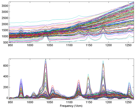
An example of the WLS Baseline method is shown in the figure below. The top plot shows the original spectra with obvious, significant baseline contributions. The bottom plot shows the same spectra following WLS Baseline application using a second-order polynomial baseline. Although some baseline features remain after baselining, the narrow Raman features are much more significant contributor to the remaining signal.
Figure. Effect of Weighted Least Squares (WLS) Baselining on Raman spectra. The original data (top plot) and baseline corrected data (bottom plot) are shown.
From the command line, this method is performed using the wlsbaseline function. There is also a method called baseline which can be used to manually select the baseline points that will be used to fit a polynomial to each spectrum. The manual selection method is faster and less prone to introduction of variance, but requires more knowledge on the part of the user as to what areas of the spectra are truly baseline. In addition, there is a windowed version of the WLS baseline algorithm called baselinew. This algorithm fits an individual polynomial to multiple windows across a spectrum and is better at handling unusually shaped baselines, but requires the selection of an appropriate window size.
Baseline (Automatic Whittaker Filter)
The Automatic Whittaker Filter method is similar to the Weighted Least Squares (WLS) method described above except that it uses a piecewise method for automatically removing baseline offsets from data. It is used in the same cases as the WLS method and it conceptually does something very similar. In fact, the two methods share a settings interface because of their similarity.
There are two basic settings which are most relevant to the Whittaker filter:
- Lambda - similar to the "order" of polynomial, this setting controls the amount of curvature allowed for the baseline. The smaller the lambda, the more curvature allowed in the fit baseline.
- P - governs the extent of asymmetry required of the fit. Larger values allow more negative-going regions. Smaller values disallow negative-going regions. P must be > 0 and < 1.
From the command line, this method is performed using the wlsbaseline function with the 'filter' option set to 'whittaker'.
EEM Filtering
Excitation Emission Matrices (EEMs) are sometimes collected in fluorescence spectroscopic applications. These data sometimes require special handling to remove interferences from Rayleigh and Raman scattered light. The EEM Filtering method allows removal of these interferences by marking data down the first- and second-order Rayleigh lines and a selected Raman band as "missing". It also can optionally mark data below the first-order Rayleigh line as all zeros. In most multi-way analyses, missing data will be replaced or ignored during the model fitting.
From the command line, this method is performed using the flucut function.


