Svmda
Purpose
SVMDA Support Vector Machine (LIBSVM) for classification.
Synopsis
- model = svmda(x,y,options); %identifies model (calibration step)
- pred = svmda(x,model,options); %makes predictions with a new X-block
- pred = svmda(x,y,model,options); %performs a "test" call with a new X-block and known y-values
Description
SVMDA performs calibration and application of Support Vector Machine (SVM) classification models. (Please see the svm function for support vector machine regression problems). These are non-linear models which can be used for classification problems. The model consists of a number of support vectors (essentially samples selected from the calibration set) and non-linear model coefficients which define the non-linear mapping of variables in the input x-block to allow prediction of the classification as passed in either as the classes field of the x-block or in a y-block which contains integer-valued classes. It is recommended that regression be done through the svm function.
Svmda is implemented using the LIBSVM package which provides both cost-support vector regression (C-SVC) and nu-support vector regression (nu-SVC). Linear and Gaussian Radial Basis Function kernel types are supported by this function.
Note: Calling svmda with no inputs starts the graphical user interface (GUI) for this analysis method.
Inputs
- x = X-block (predictor block) class "double" or "dataset", containing numeric values,
- y = Y-block (predicted block) class "double" or "dataset", containing integer values,
- model = previously generated model (when applying model to new data).
Outputs
- model = a standard model structure model with the following fields (see MODELSTRUCT):
- modeltype: 'SVM',
- datasource: structure array with information about input data,
- date: date of creation,
- time: time of creation,
- info: additional model information,
- pred: 2 element cell array with
- model predictions for each input block (when options.blockdetail='normal' x-block predictions are not saved).
- detail: sub-structure with additional model details and results, including:
- model.detail.svm.model: Matlab version of the libsvm svm_model (Java)
- model.detail.svm.cvscan: results of CV parameter scan
- model.detail.svm.outlier: results of outlier detection (one-class svm)
- pred a structure, similar to model for the new data.
- pred: The vector pred.pred{2} will contain the class predictions for each sample.
Options
options = a structure array with the following fields:
- display: [ 'off' | {'on'} ], governs level of display to command window,
- plots [ 'none' | {'final'} ], governs level of plotting,
- preprocessing: {[]} preprocessing structures for x block (see PREPROCESS). NOTE that y-block preprocessing is NOT used with SVMDA. Any y-preprocessing will be ignored.
- blockdetails: [ {'standard'} | 'all' ], extent of predictions and residuals included in model, 'standard' = only y-block, 'all' x- and y-blocks.
- algorithm: [ 'libsvm' ] algorithm to use. libsvm is default and currently only option.
- kerneltype: [ 'linear' | {'rbf'} ], SVM kernel to use. 'rbf' is default.
- svmtype: [ {'c-svc'} | 'nu-svc' ] Type of SVM to apply. The default is 'c-svc' for classification.
- probabilityestimates: [0| {1} ], whether to train the SVR model for probability estimates, 0 or 1 (default 1)"
- cvtimelimit: Set a time limit (seconds) on individual cross-validation sub-calculation when searching over supplied SVM parameter ranges for optimal parameters. Only relevant if parameter ranges are used for SVM parameters such as cost, epsilon, gamma or nu. Default is 10 (seconds);
- splits: Number of subsets to divide data into when applying n-fold cross validation. Default is 5.
- gamma: Value(s) to use for LIBSVM kernel gamma parameter. Default is 15 values from 10^-6 to 10, spaced uniformly in log.
- cost: Value(s) to use for LIBSVM 'c' parameter. Default is 11 values from 10^-3 to 100, spaced uniformly in log.
- nu: Value(s) to use for LIBSVM 'n' parameter (nu of nu-SVC, and nu-SVR). Default is the set of values [0.2, 0.5, 0.8].
- outliernu: Value to use for nu in LIBSVM's one-class svm outlier detection. A negative value disables outlier detection and it is disabled by default. It is enabled by setting outliernu to a positive value, for example outliernu=0.05.
Algorithm
Svmda uses the LIBSVM implementation using the user-specified values for the LIBSVM parameters (see options above). See [1] for further details of these options.
The default SVMDA parameters cost, nu and gamma have value ranges rather than single values. This svm function uses a search over the grid of appropriate parameters using cross-validation to select the optimal SVM parameter values and builds an SVM model using those values. This is the recommended usage. The user can avoid this grid-search by passing in single values for these parameters, however.
C-SVC and nu-SVC
There are two commonly used versions of SVM classification, 'C-SVC' and 'nu-SVC'. The original SVM formulations for Classification (SVC) and Regression (SVR) used parameters C [0, inf) and epsilon[0, inf) to apply a penalty to the optimization for points which were not correctly separated by the classifying hyperplane or for prediction errors greater than epsilon. Alternative versions of both SVM classification and regression were later developed where these penalty parameters were replaced by an alternative parameter, nu [0,1], which applies a slightly different penalty. The main motivation for the nu versions of SVM is that it has a has a more meaningful interpretation. This is because nu represents an upper bound on the fraction of training samples which are errors (misclassified, or poorly predicted) and a lower bound on the fraction of samples which are support vectors. Some users feel nu is more intuitive to use than C or epsilon. C/epsilon or nu are just different versions of the penalty parameter. The same optimization problem is solved in either case. Thus it should not matter which form of SVM you use, C versus nu for classification or epsilon versus nu for regression. PLS_Toolbox uses the C and epsilon versions since these were the original formulations and are the most commonly used forms. For more details on 'nu' SVMs see [2]
Class prediction probabilities
LIBSVM calculates the probabilities of each sample belonging to each possible class. The method is explained in [3], section 8, "Probability Estimates". PLS_Toolbox provides these probability estimates in model.detail.predprobability or predict.detail.predprobability, which are nsample x nclasses arrays. The columns are the classes, in the order given by model.detail.svm.model.label (or prediction.detail.svm.model.label), where the class values are what was in the input X-block.class{1} or Y-block. These probabilities are used to find the most likely class for each sample and this is saved in pred.pred{2} and model.detail.predictedclass. This is a vector of length equal to the number of samples with values equal to class values (model.detail.class{1}).
SVMDA Parameters
- cost: Cost [0 ->inf] represents the penalty associated with errors. Error refers to a sample which do not lie on the proper side of the margin for that sample's class. Increasing cost value causes closer fitting to the calibration/training data and usually a narrower margin width. nu is not required if cost is specified.
- gamma: Kernel gamma parameter controls the shape of the separating hyperplane. Increasing gamma usually increases number of support vectors.
- nu: Nu (0 -> 1] is an alternative parameter for specifying the penalty associated with errors. It indicates a lower bound on the number of support vectors to use, given as a fraction of total calibration samples, and an upper bound on the fraction of training samples which are errors (misclassified). cost is not required if nu is specified.
Examples of SVMDA models on simple two-class data
The effects of the cost, gamma and nu parameters on SVMDA are examined by applying SVMDA to a simple two-variable (x,y) dataset where 100 samples belong to red class and 100 to blue class. This is equivalent to an X-block having dimensions 200x2. The data are distributed as three clusters, two red clusters with 50 points each which lie nearly on either side of a blue cluster which has 100 points. SVMDA attempts to draw a dividing line between these clusters separating the x-y domain into red and blue regions. It uses these calibration data points to find the optimal separating decision boundary (hyperplane) with the widest separating margin. Any future test samples will be classified as red or blue according to which side of the separating boundary they occur on. The following images show SVMDA classification models trained on these data using an RBF kernel and varying values for the cost, gamma and nu parameters. Note that an SVMDA model with linear kernel cannot be a good model for this dataset since the red and blue points cannot be separated by a straight line, linear boundary.
- Fig. 1. Two-class dataset
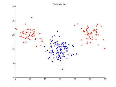
Two-variable data with 100 red samples and 100 blue samples.

The following figures show SVMDA model results where the decision boundary is shown as a black contour line. The margin edges are shown by blue and red contours. Data points which are support vectors are marked by an enclosing circle. Data points which lie on the wrong side of the decision boundary are marked with an 'x'.
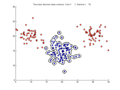
Effect of varying cost parameter for SVMDA using RBF kernel
Fig. 2a-d show the effect of increasing the cost parameter from 0.1 to 100 while gamma is kept fixed = 0.01. When the cost is small. Fig. 2a, the margin is wide since there is a small penalty associated with data points which are within the margin. Note that any point which lies within the margin or on the wrong side of the decision boundary is a support vector. Increasing the cost parameter leads to a narrowing of the margin width and fewer data points remaining within the margin, until cost = 100 (Fig. 1d) where the margin is narrow enough to avoid having any points remain inside it. Further increases in cost have no effect on the margin since no data points remain to be penalized. At the other extreme, when cost is reduced to 0.01 or smaller, the margin expands until it encloses all the data points, so all points are support vectors. This is undesirable since fewer support vectors make a more efficient model when predicting for new data points. The separating boundary in all these cases approximately keeps the same nice smooth contour as in Fig. 2a so overfitting the calibration data is not an issue in this simple case. If there was more overlapping of the red and greed data points then larger cost parameter would cause the separating boundary to deform slightly and the margin edges to be much more contorted as it tries to exclude data points from the margin.
- Fig. 2. Effect of varying cost parameter, with gamma = 0.01
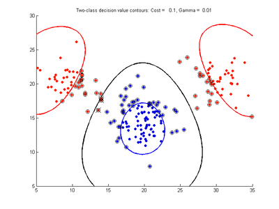
a) cost = 0.1
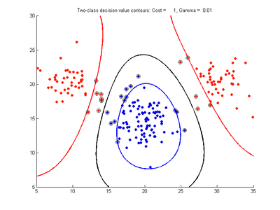
b) cost = 1.0
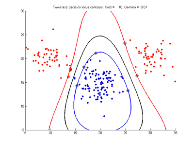
c) cost = 10

d) cost = 100


Effect of varying gamma parameter for SVMDA using RBF kernel
Fig. 3a-f show the effect of changing the gamma parameter while cost is held fixed = 1.0. These show that gamma has a major effect on how smooth or contorted the decision boundary will be, with smaller values of gamma creating a smoother decision boundary. Fig3a shows the decision boundary to be nearly linear, showing that the SVM with RBF kernel tends to approximate the linear kernel for small gamma values. At large gamma values, however, the decision boundary becomes more contorted and shows how the SVM can overfit the calibration data. The SVM in Fig. 3f produces a decision boundary which would not be a very good class predictor for the class of new test data samples.
- Fig. 3. Effect of varying gamma parameter, with cost = 1.0
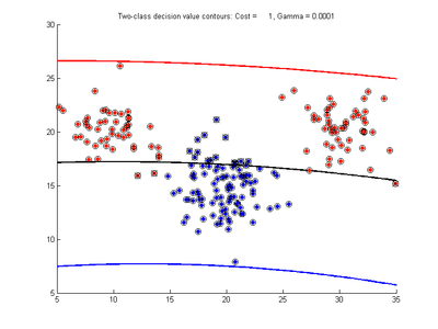
a) gamma = 0.0001
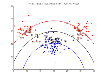
b) gamma = 0.001
c) gamma = 0.01
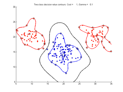
d) gamma = 0.1
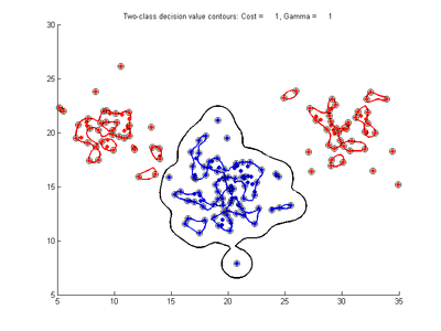
e) gamma = 1.0
f) gamma = 10.0


In summary, these comparisons show that the gamma parameter controls how smooth the decision boundary will be, with larger gamma producing more more complicated boundaries, while the cost parameter controls the width of the separating margin, with larger values of cost making the margin narrower.
Effect of varying nu parameter for SVMDA using RBF kernel
Fig. 4a-d show the effect of decreasing the nu parameter from 0.5 to 0.01 while gamma is kept fixed = 0.01. These figures show that decreasing nu has the same effect as was obtained by increasing the cost parameter, that is, it causes the margin width to decrease. It shows how nu is simply a different representation of the cost penalty parameter. The reason for its use is that its value can be interpreted as a lower bound on the number of samples which are support vectors, and also as an upper bound on the number of misclassification errors.
- Fig. 4. Effect of varying nu parameter, with gamma = 0.01
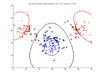
a) nu= 0.5
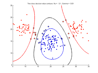
b) nu = 0.1
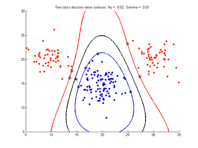
c) nu = 0.02
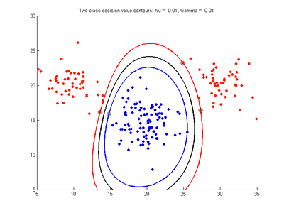
d) nu = 0.01


