Fitpeaks
Purpose
Peak fitting routine.
Synopsis
- [peakdefo,fval,exitflag,out,fit,res] = fitpeaks(peakdef,y,ax,options)
Description
Based on the initial guess in input peakdef, FITPEAKS estimates the peak fit (also the Jacobian and Hessian), and makes a call to LMOPTIMIZEBND to find the best fit of the peaks to the data. (See LMOPTIMIZEBND for additional information.) Results are output to peakdefo.
Information about individual peaks is stored in standard peak structures (see PEAKSTRUCT). Information on multiple peaks is stored in a multi-record structure. Given a standard peak structure peakdef that contains an initial guess of peak locations and widths, FITPEAKS finds new parameters that best fits peaks to the rows of the data matrix y. Results are output to a standard peak structure peakdefo.
Fields of peakdef required in the initial guess for each peak are .fun, .param, .lb, .penlb, .ub, and .penub.
Inputs
- peakdef = multi-record standard peak structure with the following fields:
- name: 'Peak', name indicating that this is a standard peak structure.
- id: ' ', double or character string peak identification.
- fun: [ {'Gaussian'} | 'Lorentzian' | 'PVoigt1' | 'PVoigt2' ], defines the peak function (see definitions in the Algorithm section).
- param: Parameter list for each peak function. The number of parameters depends on the peak function used:
- 'Gaussian': [height, location, width] (width is expressed as standard deviation - multiply by 2*sqrt(2*(-log(0.5))) = 2.3548 to calculate full-width at half-height.)
- 'Lorentzian': [height, location, width] (width is expressed as half-width - multiply by 2 to calculate full-width at half-height.)
- 'PVoigt1': [height, location, width, fraction Gaussian]
- 'PVoigt2': [height, location, width, fraction Gaussian]
- 'GaussianSkew': [height, location, width, skewparameter]
- lb: [ ], Lower bounds on the function parameters. This is a row vector with the same number of elements as peakdef.param.
- penlb: [ ], Penalty wt for lower bounds, >=0. This is a row vector with the same number of elements as peakdef.param. If set to 0 this constraint is not employed.
- ub: [ ], Upper bounds on the function parameters. This is a row vector with the same number of elements as peakdef.param.
- penub: [ ], Penalty wt for upper bounds, >=0. This is a row vector with the same number of elements as peakdef.param. If set to 0 this constraint is not employed.
- area: [ ], Estimated peak area.
- y = MxN measured responses with peaks to fit. Each row of (y) is fit to the peaks given in (peakdef).
Optional Inputs
- ax = 1xN x-axis to fit to {default ax=1:N}.
- options = discussed below in the Options Section.
Outputs
- peakdefo = The input peak structure peakdef with parameters changed to correspond to the best fit values.
- fval = Scalar value of the objective function evaluated at termination of FITPEAKS.
- exitflag = Describes the exit condition (see LMOPTIMIZEBND).
- out = Structure array with information on the optimization/fitting (see LMOPTIMIZEBND).
- fit = Model fit of the peaks, i.e it is the best fit to y.
- res = Residuals of fit of the peaks.
Algorithm
Peaks are fit to the functions defined below based on the definitions in the field (peakdef.fun). The functions can be evaluated using independent functions or a wrapper function PEAKFUNCTION. See PEAKFUNCTION for more help.
For peakdef.fun = 'Gaussian' the function is
where is the ith element of optional input ax, and corresponds to the peak parameters in the three-element vector peakdef.param. Constraints that should be used are (bounds in peakdef) are and .
For peakdef.fun = 'Lorentzian' the function is
Constraints that should be used are (bounds in peakdef) are and .
For peakdef.fun = 'PVoigt1' the function is
where corresponds to the peak parameters in the four-element vector peakdef.param. Constraints that should be used are (bounds in peakdef) are and , while . The Pseudo-Voigt peak shape is an estimate of the Gaussian and Lorentzian peak shapes convolved.
For peakdef.fun = 'PVoigt2' the function is
where corresponds to the peak parameters in the four-element vector peakdef.param. Constraints that should be used (bounds in peakdef) are and , while . The Pseudo-Voigt peak shape is an estimate of the Gaussian and Lorentzian peak shapes convolved.
For peakdef.fun = 'GaussianSkew' (a skewed Gaussian) the function is
- Failed to parse (SVG (MathML can be enabled via browser plugin): Invalid response ("Math extension cannot connect to Restbase.") from server "https://wikimedia.org/api/rest_v1/":): {\displaystyle f\left( \mathbf{x} \right)={{x}_{1}}{{e}^{\tfrac{-{{\left( x-{{x}_{2}} \right)}^{2}}}{2x_{3}^{2}}}}\int_{-\infty }^{{{x}_{4}}\left( \tfrac{x-{{x}_{2}}}{{{x}_{3}}} \right)}{{{e}^{\tfrac{-{{t}^{2}}}{2}}}dt}}
where corresponds to the peak parameters in the four-element vector peakdef.param. Constraints that should be used (bounds in peakdef) are and . The peak area is .
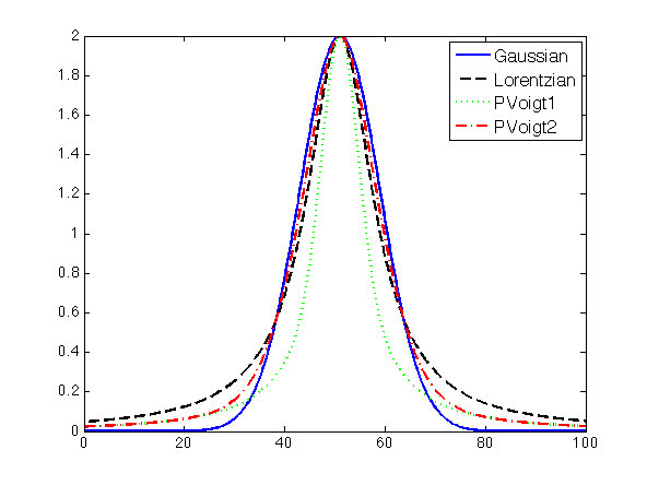
A comparison of the first four peaks is given in the figure below, and was generated using the following code:
  ax     = 0:0.1:100;
  y      = zeros(4,length(ax));
  plot(ax,peakgaussian([2 51 8],ax),'-b', ...
       ax,peaklorentzian([2 51 8],ax),'--k', ...
       ax,peakpvoigt1([2 51 8 0.5],ax),':g', ...
       ax,peakpvoigt2([2 51 8 0.5],ax),'-.r')
  legend('Gaussian','Lorentzian','PVoigt1','PVoigt2')
Options
options = structure array with the following fields:
- name: 'options', name indicating that this is an options structure.
- display: [ 'off' | {'on'} ] governs level of display to the command window.
- optimopts: options structure from LMOPTIMIZEBND. This field is passed to LMOPTIMIZEBND and can be used to control the optimization / fitting.
Examples
%Make a single known peak
ax            = 0:0.1:100;
y             = peakgaussian([2 51 8],ax);

%Define first estimate and peak type
peakdef       = peakstruct;
peakdef.param = [0.1  43   5]; %coef, position, spread
peakdef.lb    = [0     0  0.0001]; %lower bounds on param
peakdef.penlb = [1e-6 1e-6 1e-6];
peakdef.ub    = [10 99.9 40]; %upper bounds on params
peakdef.penub = [1e-6 1e-6 1e-6];

%Estimate fit and plot
yint   = peakfunction(peakdef,ax);
[peakdef,fval,exitflag,out] = fitpeaks(peakdef,y,ax);
yfit   = peakfunction(peakdef,ax); figure
plot(ax,yint,'m',ax,y,'b',ax,yfit,'r--')
legend('Initial','Actual','Fit')
See Also
peakfind, lmoptimizebnd, peakfunction, peakgaussian, peaklorentzian, peakpvoigt1, peakpvoigt2, peakstruct


![{\displaystyle \scriptstyle \mathbf {x} =\left[x_{1}\;x_{2}\;x_{3}\right]}](https://wikimedia.org/api/rest_v1/media/math/render/svg/f639c8eb1436c4ecc6149801f3b2628f8b5b44b5)


![{\displaystyle f(a_{i},\mathbf {x} )=x_{1}\left[1+\left({\frac {a_{i}-x_{2}}{x_{3}}}\right)^{2}\right]^{-1}=x_{1}\left[{\frac {\left(x_{3}\right)^{2}}{\left(x_{3}\right)^{2}+\left(a_{i}-x_{2}\right)^{2}}}\right]}](https://wikimedia.org/api/rest_v1/media/math/render/svg/2f1a4640f3bb770c5635d9d1f518e5a0de1e9d7f)
![{\displaystyle f(a_{i},\mathbf {x} )=x_{1}\left[x_{4}\exp \left({\frac {-4\ln(2)\left(a_{i}-x_{2}\right)^{2}}{\left(x_{3}\right)^{2}}}\right)+\left(1-x_{4}\right)\left[{\frac {\left(x_{3}\right)^{2}}{\left(a_{i}-x_{2}\right)^{2}+\left(x_{3}\right)^{2}}}\right]\right]}](https://wikimedia.org/api/rest_v1/media/math/render/svg/5c09ce83b13f8f321aaf0dc4a37f60b9ced0bf3d)
![{\displaystyle \scriptstyle \mathbf {x} =\left[x_{1}\;x_{2}\;x_{3}\;x_{4}\right]}](https://wikimedia.org/api/rest_v1/media/math/render/svg/cf19382b4dfcee92328e902d32fa13b7691f931d)

![{\displaystyle f(a_{i},\mathbf {x} )=x_{1}\left[x_{4}\exp \left({\frac {-\left(a_{i}-x_{2}\right)^{2}}{2\left(x_{3}\right)^{2}}}\right)+\left(1-x_{4}\right)\left[{\frac {\left(x_{3}\right)^{2}}{\left(a_{i}-x_{2}\right)^{2}+\left(x_{3}\right)^{2}}}\right]\right]}](https://wikimedia.org/api/rest_v1/media/math/render/svg/cf8ee44dcf3718fe54d841f1feda42c8199131d3)

