Multi-block Multi-set and Data Fusion
Introduction
This page gives an overview of combining data blocks in PLS_Toolbox and Solo. There are various reasons for joining multiple data blocks together, and multiple ways in which they can be joined. Some typical examples include:
- Adding samples to an existing set of data to improve a calibration data set
- Combining data from different experiments measured using the same technique(s) (data fusion)
- Combining multiple measurements taken on the same objects (aka samples) or over the same or similar periods of time (for a time-dependent system) (multi-block)
- Examining the relationship between measurement techniques for a given set of samples
- Determining the effect of one or more experimental factors on a system (multi-set and multi-level)
The joining procedures and the use of sample-wise joined data in multi-set and multi-level analyses are described below.
Joining Data
In most cases, the join procedure tends to use one of two approaches:
- Joining the data blocks as new objects or samples over the same or similar measured variables
- Joining the data blocks as new variables for the same or similar objects or samples
Joining As New Samples
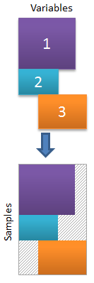
Joining as new samples is often a fairly simple process in that new data is simply appended on as new rows to a data matrix. In general, the number and type of variables must match, but tools (matchvars) exist that handle alignment of the different variable sets. Schematically, the process is shown in the image below. The gray areas are regions of "missing data" where the given block didn't have values for the specific variables.
The practical task of joining a second data block (or multiple additional data blocks) on as new samples can be accomplished within the Workspace Browser, Analysis Window, or DataSet Editor windows by simply dragging the new data files or loaded data object (usually from Workspace Browser) onto the existing loaded data. When dropped, you will be asked if you want to join the data as new samples, variables, or sometimes as new "slabs" (for 3D data). (The options available depend on the size of the data and only "Samples" may be available if sizes don't generally match.) The alignment of variables will generally be handled automatically and the blocks will be joined.
From the Matlab command line with PLS_Toolbox, the DataSet method augment() can be used to do joins:
newdata = augment(1,data1,data2,data3)
would join three data blocks (data1, data2, data3) in the first mode (samples) automatically handling the variable alignment. The "1" as the first input to this command indicates to join in the first mode (samples).
Joining as New Variables
Joining data blocks as new variables is often more complex task and usually involves at least a scaling of the blocks (correcting for magnitude and variance). Sometimes the join involves additional block-specific preprocessing or even decomposing or analyzing the block with a multivariate model and using the outputs of that model in the join. Conceptually, the simplest join is shown below.
Although a drag-drop approach to joining data blocks can be used as with samples (discussed above), the better solution to these operations is to use the Multiblock Tool which handles the various alignment, scaling, preprocessing, and modeling options. The details of this tool are discussed on the Multiblock Tool page.
Multi-Set and Multi-Level Data Analysis
Multi-set data (multi-group, etc) in PLS_Toolbox/Solo are datasets where samples are organized into sub-sets. Such datasets can be used in any analysis method with the sample grouping information used passively as a labeling or actively to represent class membership and be used to build classification models.
There is an important special case where the data were measured following a designed experiment (DOE) plan and the subsetting indicates the different DOE factor levels of the samples. PLS_Toolbox/Solo includes two methods which are intended for analyzing such multi-set datasets, ANOVA-Simultaneous Component Analysis (ASCA) and Multi-level Simultaneous Component Analysis (MLSCA).
ASCA is intended for use on crossed (factorial) DOE datasets. It isolates the variability associated with each factor and interaction and measures the significance of these. See ASCA.
MLSCA is intended for nested DOE datasets. It finds the variability of the level-averaged data ("between" variability) and the the inherent ("within") variability where the confounding effects of the factor level means are removed. See MLSCA.

